This individual course project studies loss prediction across learning-rate schedules. Given a fixed MPL baseline and one observed cosine training curve, I estimate a residual correction for WSD-family schedules. Calibration does not use target WSD losses.

Code, data manifest, and reproduction instructions · Numerical results

Problem

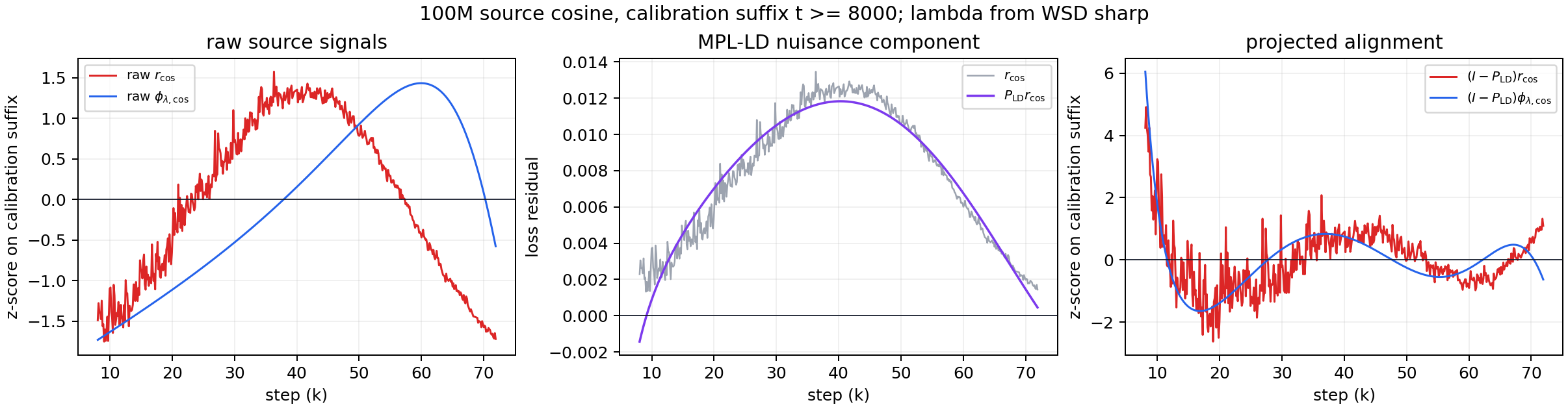
The project uses public loss-curve CSV files. It does not train new Transformers. The baseline leaves a structured residual on the source cosine curve. This residual contains both a learning-rate-drop response and drift caused by the baseline’s learning-rate-dependent parameters. Transferring the full residual can therefore transfer error that does not apply to the target schedule.

Identification problem

The central decomposition in the report is:

• a transferable LR-drop response
• non-transferable MPL-LD parameter drift
• smaller residual noise and unmodeled structure

The identification step is to remove the local MPL-LD tangent directions before estimating the response amplitude. After that projection, I fit only one nonnegative scalar from the source cosine residual. The target schedule then supplies the response shape.

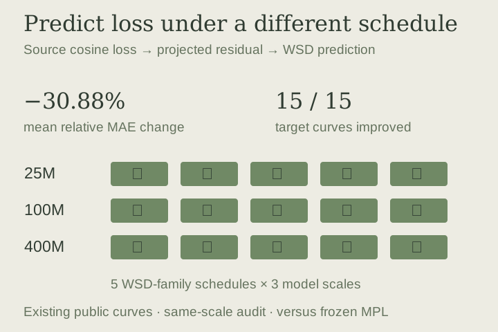
Redrawn from the robustness audit. Each marked cell is an evaluated target curve; this is a result summary, not a plotted training trajectory.

The estimator

The deployable predictor is intentionally small:

$$
\hat L_s(t)=L_{\mathrm{MPL},s}(t)+a_s\hat\kappa_s\phi_{\lambda_s,s}(t).
$$

Here $L_{\mathrm{MPL},s}$ is the frozen MPL prediction. The response feature $\phi_{\lambda_s,s}$ is a causal convolution of positive learning-rate drops. The response rate $\lambda_s$ is chosen from a schedule-only $q_2$ drop-concentration statistic, and the locality factor $a_s$ suppresses diffuse full-horizon schedule modes. The only quantity fit from loss residuals is $\hat\kappa_s$, and it is fit on the source cosine curve after the MPL-LD nuisance projection.

Calibration uses the source cosine loss. Feature construction uses the target schedule. Target losses are used only to evaluate the completed prediction.

What the audit shows

The public audit table evaluates three model scales (25M, 100M, and 400M), with five WSD-family target curves per scale. Target losses are used for evaluation, not amplitude calibration.

Evaluation	Mean relative MAE change vs. MPL	Improved target curves
Projected correction, same scale	−30.88%	15 / 15
Same-scale control without nuisance projection	+625.92%	0 / 15
Leave-one-scale-out mean-amplitude transfer	−25.62%	15 / 15

A negative change means lower error than the frozen MPL baseline. The first number is the mean of per-curve relative changes, not a pooled MAE reduction. The no-projection control supports the importance of separating baseline drift before transfer. Cross-scale success also depends on how the amplitude is aggregated: the pooled alternative worsened mean error by 62.57%.

Limits

The $q_2$ half-life rule is a schedule-derived structural prior tied to the logging resolution, not a theorem about optimizer dynamics. The calibration suffix is chosen by a source-only identifiability rule, but later suffix choices still change the size of the gain. The support-projection locality explains why diffuse controls should be suppressed, but it is a boundary condition rather than a complete dynamics model.

The results are limited to the existing public loss curves. New held-out WSD schedules and new training runs are needed to test generalization beyond this dataset.

Sources

The repository contains the method, public-data manifest, and reproduction instructions. The robustness report provides the numerical results summarized above.