DLfinal

This was my final project for Mathematical Introduction to Machine Learning. The updated paper narrows the project into one question: given a frozen MPL baseline and one observed cosine training curve, can I identify a residual component that transfers to WSD-family schedules without fitting the target WSD losses?

I keep the code, paper, data manifest, and reproduction notes in GitHub / wjjpku/DL-final.

Course project framing

The paper is titled Projected LR-Drop Residuals for Source-Only Cosine-to-WSD Loss-Curve Prediction. I did not train new transformers for this project. I worked with public loss-curve CSV files, treated MPL as a frozen baseline, and asked what can be responsibly transferred from a source cosine residual.

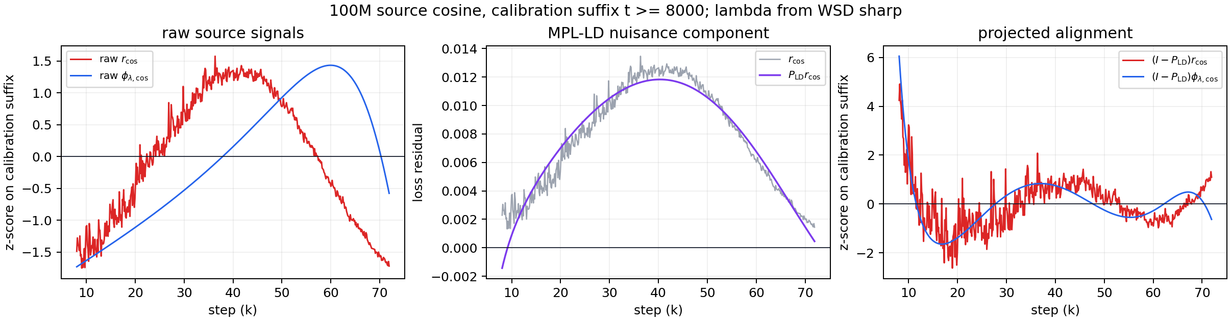
That framing matters because a raw residual is not a clean signal. In the source cosine curve, the MPL residual mixes a learning-rate-drop response with nuisance drift from MPL’s learning-rate-dependent parameters. If I transfer the raw residual directly, I am not transferring mechanism; I am copying a confounded error.

Identification problem

The central decomposition in the report is:

a transferable LR-drop response
non-transferable MPL-LD parameter drift
smaller residual noise and unmodeled structure

The identification step is to remove the local MPL-LD tangent directions before estimating the response amplitude. After that projection, I fit only one nonnegative scalar from the source cosine residual. The target schedule then supplies the response shape.

MPL residuals show structured schedule-dependent error near WSD transition and tail regions

The estimator

The deployable predictor is intentionally small:

$$
\hat L_s(t)=L_{\mathrm{MPL},s}(t)+a_s\hat\kappa_s\phi_{\lambda_s,s}(t).
$$

Here (L_{\mathrm{MPL},s}) is the frozen MPL prediction. The response feature (\phi_{\lambda_s,s}) is a causal convolution of positive learning-rate drops. The response rate (\lambda_s) is chosen from a schedule-only (q_2) drop-concentration statistic, and the locality factor (a_s) suppresses diffuse full-horizon schedule modes. The only quantity fit from loss residuals is (\hat\kappa_s), and it is fit on the source cosine curve after the MPL-LD nuisance projection.

This is why I think of DLfinal as a residual-identification project rather than a general loss-prediction project. The method is useful only if the information boundary is kept clean: source cosine loss for calibration, target schedule for feature construction, target loss only after the prediction is finished.

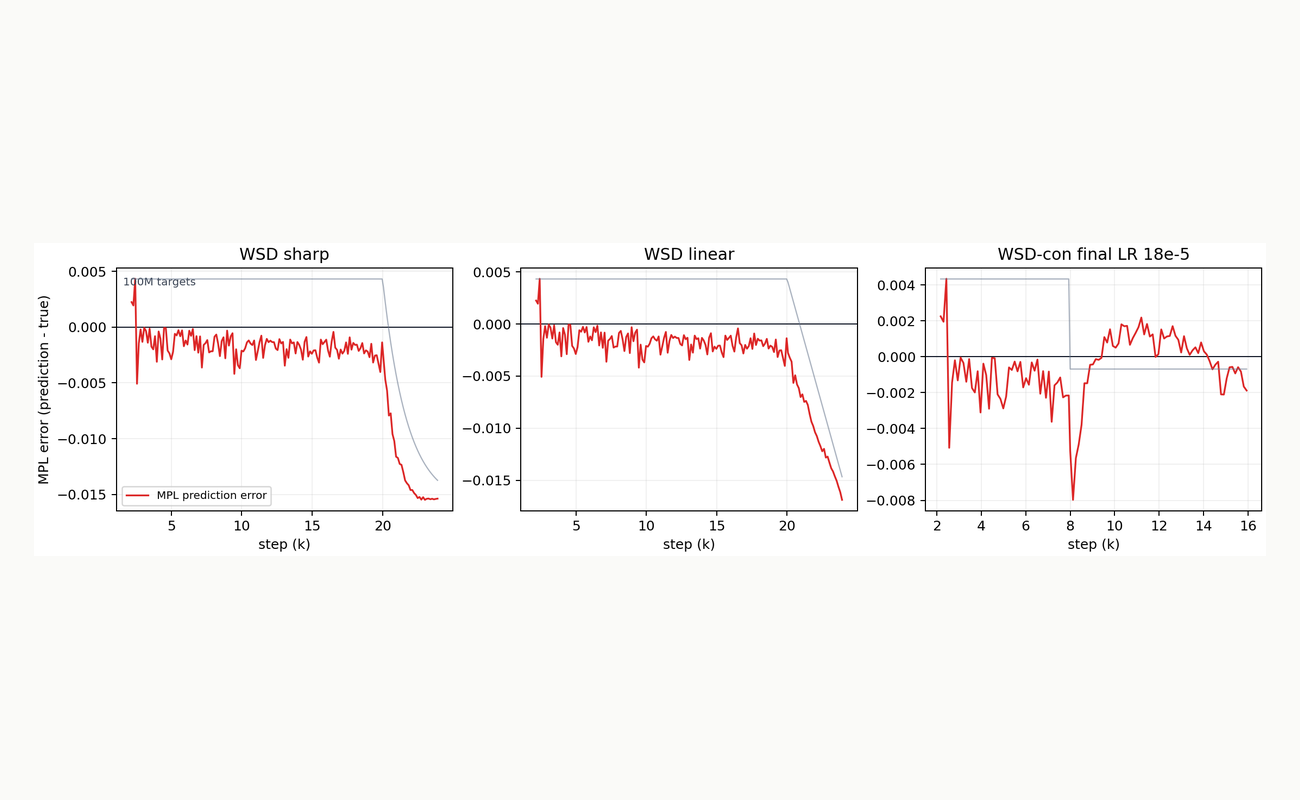
What the audit shows

The main evidence is not a single headline number. The selected formula improves every current WSD-family row in the same-scale and cross-scale audits, while the controls remain non-harmful. More importantly, the negative controls explain why the projection is necessary. A raw no-nuisance projection uses the same source residual and response idea, but fails badly because it copies MPL-LD drift along with the transferable response.

Projection separates nuisance drift from the response component I want to transfer

Limits I keep explicit

I do not present this as a universal training-loss law. The (q_2) half-life rule is a schedule-derived structural prior tied to the logging resolution, not a theorem about optimizer dynamics. The calibration suffix is chosen by a source-only identifiability rule, but later suffix choices still change the size of the gain. The support-projection locality explains why diffuse controls should be suppressed, but it is a boundary condition rather than a complete dynamics model.

The largest limitation is still external validation. The current result is strongest as a course-facing audit on the public loss-curve repository. New held-out WSD schedules or new training runs would be needed before I would claim broad generalization.

What I learned

This project made me more careful about the word “transfer.” A residual can look transferable until a negative control asks what part of it is actually being moved. The stronger habit I gained is to put the baseline first, define the information boundary second, and only then tell a mechanism story.